- Edited
The new DataDreamer v0.2.0 update expands its capabilities for generating synthetic data and pre-annotating real datasets. This version introduces SlimSAM for instance segmentation. Additionally, the Qwen 2.5 language model is now integrated as a prompt generator, boosting text data generation. With these updates, DataDreamer becomes even better suited for data preparation and annotation.
Data Prepping (Annotation)
Step 1 of training and deploying (to eg. OAK cameras) a custom ML model is data preparation. This includes collecting, cleaning, and annotating data. DataDreamer simplifies this process by providing tools for auto-annotation of images and generating synthetic data.

On the video above you can see how to use DataDreamer to auto-annotate a video (sequence of images). If you took all frames of the video
and include the in the dataset you would have a lot of similar images, which isn't good for training a model, as it would be overfitting.
That's why you'd usually take only eg. 1 frame per second, which we can accomplish easily with OpenCV (Gist here). After we have images in frames/ folder, we can use DataStreamer to auto-annotate them.
I also cropped the video (yellow rectangle) so only lemons are in the FOV (field of view), which helps with detection accuracy, as from my tests it doesn't work well with smaller objects.
Datadreamer
datadreamer --save_dir frames --class_names "lemons" --task instance-segmentation \
--annotator_size large --use_tta --image_annotator owlv2-slimsam \
--conf_threshold 0.25 --annotate_only --annotation_iou_threshold 0.1 --device cudaLet's break down the command (all Params explain here):
--save_dir frames- folder with images--class_names "lemons"- class name - I only want to detect lemons--task instance-segmentation- we want to do instance segmentation, which includes bounding boxes (detection) and masks. You could change it todetectionif you only want bounding boxes, orclassificationif you only want to classify images.annotator_size large- size of the annotator. You can choose betweenbaseandlarge.largeis more accurate, but slower.use_tta- use Test Time Augmentation. This will do rotations/flips/crops/scaling to image and aggregate predictions to make outputs more robust. It provides better results, but is slower.image_annotator owlv2-slimsam- Currently only annotator that supports segmentation.owlv2can be used for detection, andclipfor image classification.conf_threshold 0.25- confidence threshold. If the model is less than 25% sure that it's a lemon, it won't annotate it.annotate_only- just annotate images, don't generate new/synthetic data.annotation_iou_threshold 0.1- IOU threshold.device cuda- use NVIDIA GPU for inference. If you don't have a GPU, you can usecpu, but it will be much slower.
After letting it sit for a couple of minutes (or hours, depending on the number of images), you'll have annotated images in frames/annotations.json file.
erik@eriks-MacBook-Pro frames % ls -l
total 140424
-rw-r--r-- 1 erik staff 28571010 Nov 26 15:02 annotations.json
-rw-r--r-- 1 erik staff 135045 Nov 26 14:56 frame_0000.jpg
-rw-r--r-- 1 erik staff 132306 Nov 26 14:56 frame_0001.jpg
-rw-r--r-- 1 erik staff 128611 Nov 26 14:56 frame_0002.jpg
-rw-r--r-- 1 erik staff 130135 Nov 26 14:56 frame_0003.jpg
-rw-r--r-- 1 erik staff 129604 Nov 26 14:56 frame_0004.jpg
...Annotations
These are in raw format, with detections (bounding boxes), masks, and labels for each image. One could also include --dataset_format yolo or --dataset_format coco argument to get annotations in YOLO or COCO format.
Visualizing Annotations
To visualize annotations (draw mask/detection/label on the image), we'll be using SuperVision library, which is an opensource CV tool for easy visualizing and debugging computer vision models.
import cv2
import numpy as np
import json
import os
import supervision as sv
from supervision.detection.utils import polygon_to_mask
# Path to your folder containing images and annotation JSON file
image_folder = "frames"
annotation_file = "frames/annotations.json"
# Load annotations
with open(annotation_file, 'r') as f:
annotations = json.load(f)
# Sort annotations by image_name
annotations = {k: v for k, v in sorted(annotations.items(), key=lambda item: item[0])}
yellow = sv.Color(255,240,0)
label_anotator = sv.LabelAnnotator(color=yellow, text_color=sv.Color(0,0,0))
polygon_annotator = sv.PolygonAnnotator(color=yellow, thickness=3)
# Iterate through each image in the annotations
for image_name, data in annotations.items():
image_path = os.path.join(image_folder, image_name)
image = cv2.imread(image_path)
if image is None:
print(f"Could not read image: {image_name}")
continue
# Extract bounding boxes and labels from image annotation
boxes = np.array(data["boxes"], dtype=np.float32) # Bounding boxes
class_ids = np.array(data["labels"], dtype=np.int32) # Class IDs
if "masks" in data:
masks = []
for polygon in data["masks"]:
new_mask = polygon_to_mask(
polygon=np.array(polygon, dtype=np.int32),
resolution_wh=(image.shape[1], image.shape[0]) # (width, height)
)
masks.append(new_mask.astype(bool))
masks = np.array(masks, dtype=bool)
else:
masks = None
# Create sv.Detections object
if len(boxes) != 0:
detections = sv.Detections(
xyxy=boxes,
class_id=class_ids,
mask=masks
)
# Draw labels and polygons on the image
labels = ["Lemon"] * len(data["labels"]) # Only 1 class anyways
image = label_anotator.annotate(scene=image, detections=detections, labels=labels)
image = polygon_annotator.annotate(scene=image, detections=detections)
# Display the annotated image
cv2.imshow("Annotated Image", image)
cv2.waitKey(33) # Wait 33ms
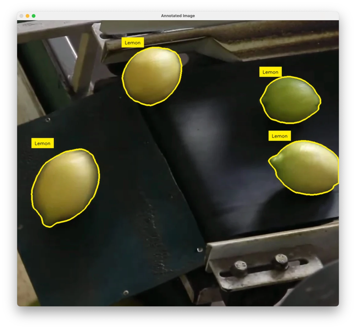
cv2.destroyAllWindows()OpenCV will open a window with the image and annotations, like on the image below. You can use q to close the window.

On the next blog post, we'll cover how to train the model and then deploy it to OAK cameras. Stay tuned!
Let us know if you have any questions/thoughts in the comments
- Erik
