In this post, we showcase a real-world use case: detecting soldering defects on SMD components using an OAK4-S edge AI camera mounted on a microscope. The OAK4-S features a 48MP IMX586 rolling shutter sensor, making it ideal for high-resolution, real-time PCB inspection.
The goal is to demonstrate how easy it is to go from an idea to an initial working prototype for edge-based defect detection, using tools like Roboflow, LuxonisTrain, and the DepthAI platform—with minimal setup and no machine learning expertise required.
While the final model still has room for improvement, the pipeline is fast, reproducible, and expandable—simply add more data or tune parameters. This workflow can be applied to any AI vision task, from PCB quality control to on-device object detection.
Whether you're targeting solder inspection, electronics manufacturing QA, or training a model for your own camera setup, this tutorial outlines a generalizable process:
From dataset → to training → to deployment on an OAK 4 device.
The Process in a Nutshell
Find a baseline dataset
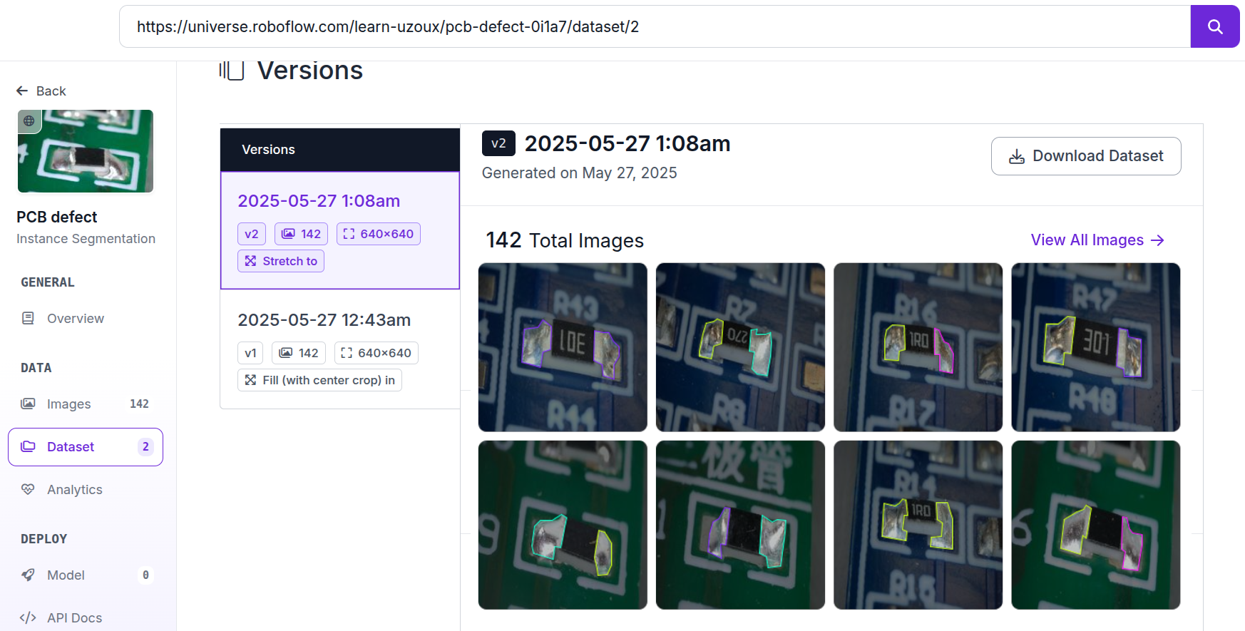
We started with a public Roboflow dataset on PCB defects. First evaluation of its performance was done on Roboflow’s web UI.
Capture and annotate our own data to add to baseline dataset
Took ~50 microscope photos with the OAK4-S and labeled defects.
Retrain the model
Combined public + custom data and trained using LuxonisTrain.
Deploy to the OAK4-S
Loaded the model onto the camera for real-time solder inspection.
Step 1: Finding and Testing a Base Model on a Public Dataset
To kick off the project, we searched for an existing dataset to jump-start development. We found a promising candidate on Roboflow Universe:
👉 PCB Defect Detection Dataset
We followed Roboflow’s steps to:
Fork the dataset.
Create a new version with preprocessing and augmentation options.
Train a baseline model directly using their web-based platform.
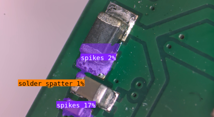
The initial results were promising but not reliable

Some obvious defects were missed, and false positives were common. The model lacked the nuance required for accurate detection under our lighting, magnification, and board types:

Step 2: Expanding with Custom Annotations
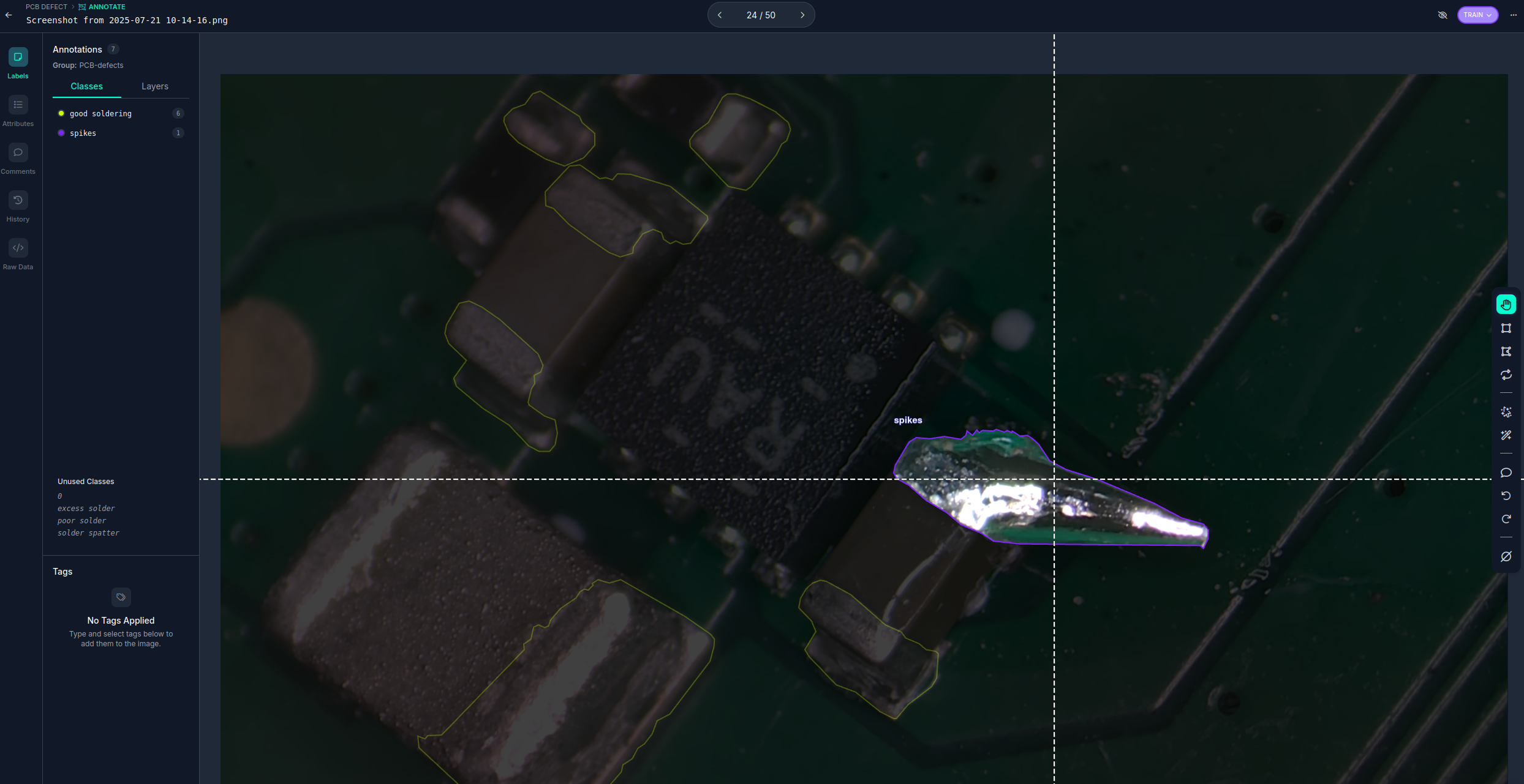
To boost performance, we captured 50+ high-resolution images of PCBs under a microscope using the OAK4-S. We manually labeled soldering conditions such as:
Solder spikes
Excess solder
Solder spatter
Good soldering

All annotations were done in Roboflow. This augmented dataset significantly improved model performance - though more diverse data (lighting, PCB types, angles) would improve generalization further.
We then generated a new dataset version that combined both the original and custom images - ready for training.

Step 3: Training the Model with LuxonisTrain
We’ve created a Jupyter-based training script that guides you through training custom models using Roboflow datasets.
👉 To continue with the tutorial, follow the steps written directly in the Jupyter notebook itself.
In the section below, we’ll focus on sharing best practices for setting up and running the training, whether you're using Google Colab or your own machine—so you can get the most out of the process.
💡Tip: This training is part of our Luxonis AI Tutorials training tools where you can find a lot of learning material for other kinds of models and datasets.
Training Setup Options
Option 1: Google Colab (Recommended for Beginners)
Colab is the easiest way to get started because everything is pre-installed and runs in the cloud:
Start with CPU runtime and set epochs: 5 in the config. This helps verify that the dataset loads and the pipeline runs correctly.
Once everything works, switch to GPU runtime for faster training.
Be mindful that free accounts have limited GPU time, so long training runs may hit resource limits.
Option 2: Local Training
If you have your own machine with a GPU, you can run the training notebook locally. The notebook installs all dependencies automatically using:
!pip install -r requirements.txt
To use your NVIDIA GPU for training, make sure you have the appropriate drivers and CUDA toolkit installed. You can find the latest versions here:
🔗 NVIDIA CUDA Toolkit
Best Practices for Training
Whether you run training on Colab or locally, here are some key principles to follow for better results:
1. Train on Deployment-Like Data
Model performance improves dramatically when trained on data that matches real deployment conditions. If accuracy is low:
Capture more images from your actual camera setup.
Annotate and add them to your dataset.
Retrain or fine-tune the model with the updated dataset.
2. Choose the Right Architecture Variant
Each model variant balances speed and accuracy differently:
Heavy → Slower but higher accuracy.
Medium → Good balance for most tasks.
Light → Fastest but with reduced accuracy.
Pick based on your application’s FPS vs accuracy needs.
3. Adjust Input Shape
Increasing the input resolution can help detect smaller features, but it will reduce FPS. If your model struggles with fine details, try a larger input shape (e.g. 512×512 or 640×640).
4. Use Smart Data Augmentations
Augmentations artificially expand dataset diversity and help generalization:
Choose augmentations that simulate your expected deployment conditions.
For example, if your dataset only contains green PCBs but the model should also work on black PCBs, consider grayscale or brightness-shift augmentations.
5. Train Until Slight Overfitting
Don’t stop training too early. Train long enough that:
Training loss keeps dropping, and
Validation loss begins to rise, signaling overfitting.
That’s your cue to stop or apply regularization.
6. Tune Learning Rate
Try experimenting with different learning rates:
Too high? Model might not converge.
Too low? Training might be unnecessarily slow or stuck.
Adjust up or down based on observed training behavior.
Step 4: Deploying to OAK4-S
Once your model is trained and uploaded to your private Luxonis Hub profile, you can deploy it to your OAK4-S camera in one of two ways: Peripheral Mode (runs on your host machine) or Standalone Mode (runs directly on the camera).
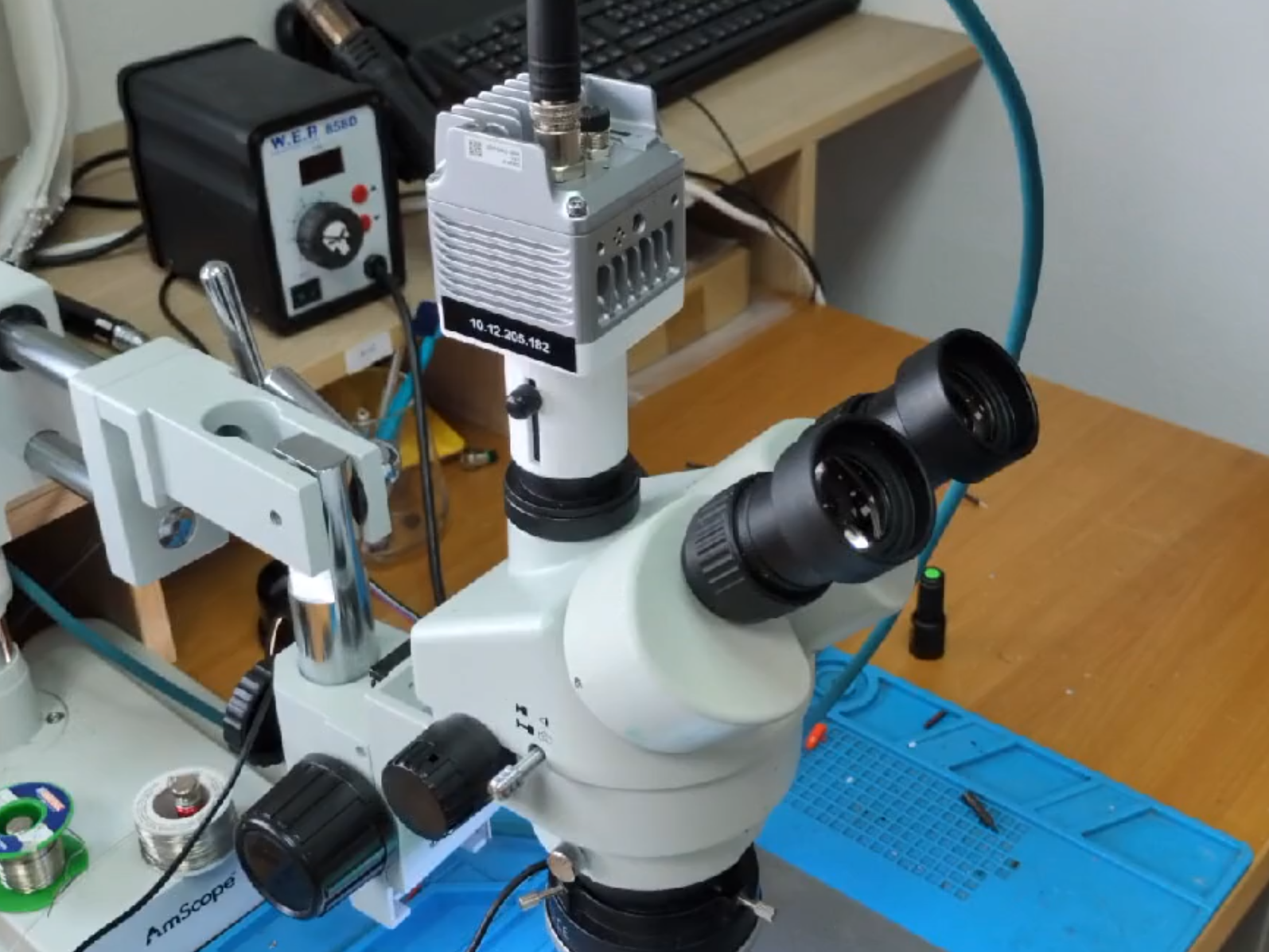
We mounted a prototype of the OAK4-S to a microscope using a custom 3D-printed holder, allowing for high-resolution inspection of SMD soldering under magnification.

💡 If you prefer to run your model directly from a local file. Follow this tutorial to learn how.
Here’s how to run Peripheral and Standalone mode with model uploaded on Luxonis Hub:
Option 1: Peripheral Mode (Quick Testing)
This is ideal for fast iteration, where the model runs on your computer but uses the OAK camera for input.
Make sure your camera is connected, and then run:
python3 neural-networks/generic-example/main.py \
-m <INSERT_MODEL_LINK_ON_LUXONIS_HUB> \
-api <INSERT_YOUR_LUXONIS_HUB_API_KEY>
-m: Model path on Luxonis Hub-api: Your Luxonis Hub API key
💡 Tip: If you’ve added your device to Luxonis Hub (via oakcli setup or through the setup.luxonis.com), you don’t need to manage an API key manually (-api <INSERT_YOUR_LUXONIS_HUB_API_KEY> does not need to be added). The key is automatically injected as the DEPTHAI_HUB_API_KEY environment variable. This simplifies authentication for testing in Peripheral Mode.
Option 2: Standalone Mode (Run Directly on Camera)
For deployment without a host computer, you can run the model fully onboard the OAK camera.
Here’s how:
- Clone the OAK examples repo:
git clone https://github.com/luxonis/oak-examples.git
- Create your secrets file
cd oak-examples/neural-networks/generic-example/ && echo "LUXONISHUB_API_KEY=<INSERT_YOUR_LUXONIS_HUB_API_KEY>" > .env
Make sure your provide your API key in the above code.
💡 Tip: We use a .env file to store the Luxonis Hub API key. This is a recommended practice to keep your credentials secure and out of version control systems like Git. See more on our Hub API key good practices docs page.
- Edit the standalone configuration:
nano oakapp.toml
- Modify the
entrypoint to include your model link and API key:
entrypoint = ["bash", "-c", "export $(cat /app/.env | xargs) && python3 -u /app/main.py --model <INSERT_MODEL_LINK_ON_LUXONIS_HUB> -api $LUXONISHUB_API_KEY --overlay"]
Make sure the --model flag contains the correct path to your model on Luxonis Hub.
- Run the standalone app on the device:
oakctl app run .
Now you will be able to see the visualization of your detections in a browser by visiting http://<IP_OF_CAMERA>:8082
Conclusion: Custom Edge AI for Real-Time PCB Inspection
With just a few tools—Roboflow, LuxonisTrain, and the OAK4-S camera—we built and deployed a custom AI model that performs on-device solder defect detection at the edge.
The same process could be applied to:
Ready to build your own AI pipeline?
📘 Explore the Luxonis AI Tutorials
🛒 Get your own OAK camera
💬 Join our community on the Forum